sar多子带点目标仿真
参数与初始化
EarthMass = 6e24; %地球质量(kg)
EarthRadius = 6.37e6; %地球半径6371km
Gravitational = 6.67e-11; %万有引力常量
f0 = 5.4e9; % 中心频率
H = 755e3; % 飞行高度
Tr = 20e-6; % 脉冲宽度
Br = 2.8e7; % 子带带宽
Fr = 1.2*Br; % 子带采样率
step_f = Br;
sub_N = 3;
sub_f = f0:step_f:f0+step_f*sub_N;

% sub_f = [sub_f2];
c = 299792458;
Vr = sqrt(Gravitational*EarthMass/(EarthRadius + H));
Vg = Vr;
Vs = Vr;
La = 12;
phi = deg2rad(20); % 俯仰角
incidence = deg2rad(20.5); % 入射角

Kr = Br/Tr;
sub_lambda = c./sub_f;
lambda = c/(f0+step_f*sub_N/2);


R0 = H/cos(phi);
R_eta_c = H/cos(incidence);
theta_rc = acos(R0/R_eta_c);
eta_c = -R_eta_c*sin(theta_rc)/Vr;

sub_fnc = 2*Vr*sin(theta_rc)./sub_lambda;
fnc = 2*Vr*sin(theta_rc)/lambda;
Ta = 0.886*R_eta_c*lambda/(La*Vg*cos(theta_rc));
delta_fdop = 2*0.886*Vs*cos(theta_rc)/La;
PRF = 1.7*delta_fdop;
% Ka = 2*Vr^2*cos(theta_rc)^3/(lambda*R0);

Nr = 2*ceil(Fr*Tr);
Na = 2*ceil(PRF*Ta);

% 构造距离向与方位向时间与频率
t_tau = 2*R_eta_c/c + (-Nr/2:Nr/2-1)*(1/Fr);
t_eta = eta_c+(-Na/2:Na/2-1)*(1/PRF);


f_tau = fftshift((-Nr/2:Nr/2-1)*(Fr/Nr));
f_eta = fnc+(-Na/2:Na/2-1)*(PRF/Na);

[mat_t_tau, mat_t_eta] = meshgrid(t_tau, t_eta);
[mat_f_tau, mat_f_eta] = meshgrid(f_tau, f_eta);

% 脉内串发,构造偏移时间
step_T = 1/PRF;
sub_t_offset = (0:sub_N-1)*step_T; % 添加保护带,偏移时间为2*T
参数设置这里需要注意精度与测绘宽度之间的协调,不然容易爆内存(如果用自己的电脑仿真)。
距离向精度主要与信号带宽有关,满足
这里 $\gamma$ 为展宽,如果没有加窗,设为1就行。距离向的最大测绘宽度主要与脉冲宽度有关,与脉冲宽度成正比。方位向精度为
\[\rho_a \approx \frac{L_a}{2}\]方位向测绘宽度与目标照射时间有关,如果想不影响方位向精度,调宽度,可以调雷达高度。 子带发射有三种模式
- 脉间串发:子带偏移时间为 $1/PRF$ 。
- 脉内串发:子带偏移时间为 $t_{offset} > T_r$
- 脉内并发:子带同时发射,偏移时间为0。
需要注意的是各个子带的多普勒中心不一样,每个子带的多普勒中心需要单独算。 看完论文,对于成像我大致有两个想法
- 距离压缩->子带合成->RCMC->方位压缩
- 距离压缩->RCMC->方位压缩->子带合成 这两种,我均有尝试,效果差别很大。
点目标回波产生
pointx = 0;
pointy = 0;
point = [pointx, pointy];

S_echo = zeros(3, Na, Nr);
noisy_A = randn([1,sub_N]);
noisy_P = randn([1,sub_N])*2;
noisy_T = randn([1,sub_N])*5*1e-9;

% noisy_A = zeros(1,sub_N);
% noisy_P = zeros(1,sub_N);
% noisy_T = zeros(1,sub_N);

for i = 1:sub_N

    mat_t_tau_noisy = mat_t_tau - noisy_T(i);
    mat_t_eta_offset = mat_t_eta+sub_t_offset(i);

    R0_target = sqrt((R0*sin(phi)+point(1))^2+H^2);
    R_eta_target = sqrt(R0_target^2+(point(2)-Vr*mat_t_eta_offset).^2);
    t_etac_target = (point(2)-R0_target*tan(theta_rc))/Vr;

    Wr = (abs(mat_t_tau_noisy-2*R_eta_c/c) < Tr/2);
    % Wa = sinc((La*atan(Vg*(mat_t_eta_offset - t_etac_target)./R0_target)/sub_lambda(i))).^2;
    Wa = abs(mat_t_eta_offset - eta_c - sub_t_offset(i))<Ta/2;
    sub_phase = exp(1j*pi*Kr*(mat_t_tau_noisy-2*R_eta_target/c).^2).*exp(-2j*pi*sub_f(i)*2*R_eta_target/c).*exp(2j*pi*noisy_P(i));

    S_echo(i,:,:) = (1+noisy_A(i))*Wr.*Wa.*sub_phase;
end
在回波产生时,对每个子带添加随机扰动。其他与一般的sar回波产生无区别。
距离压缩->RCMC->方位压缩->子带合成
距离压缩
    sub_S_echo = squeeze(S_echo(i, :, :));
    Hr =  (abs(mat_f_tau)<Br/2).*exp(1j*pi*mat_f_tau.^2/Kr);
    sub_S_ftau_eta = fft(sub_S_echo, Nr, 2);
    sub_S_ftau_eta = sub_S_ftau_eta.*Hr;
对每个子带进行相同的距离压缩操作,没什么需要注意的。需要注意的是后续的对每个子带的补偿操作
    R_eta = sqrt(R0^2+(Vr*(mat_t_eta+sub_t_offset(i))).^2);
    sub_S_ftau_eta = sub_S_ftau_eta.*exp(-2j*pi*2*(R_eta-R_ref)/c.*mat_f_tau);%补偿串发导致的斜距差

    sub_S_tau_eta = ifft(sub_S_ftau_eta, Nr, 2);

    sub_S_tau_eta = sub_S_tau_eta.*exp(2j*pi*(fnc-sub_fnc(i)).*mat_t_eta); %移动多普勒中心

    sub_S_tau_feta = fft(sub_S_tau_eta, Na, 1);
    sub_S_tau_feta = sub_S_tau_feta.*exp(-2j*pi*mat_f_eta*sub_t_offset(i)); %方位向补偿时延
首先需要做的是补偿串发导致的斜距差,斜距差导致时延不同。这里斜距差大致在分米级,如果成像在厘米级,是必须要补偿的。但如果精度为米级,则无需考虑,方位向的时延也类似。 多普勒中心是必须要移动的,保证每个子带的多普勒中心在一个位置,没有可能会加重栅瓣的影响。
RCMC与方位压缩
对每个子带进行R距离徙动校正与方位压缩。
    mat_f_eta_offset = mat_f_eta;
    delta_R = lambda^2*R0*mat_f_eta_offset.^2/(8*Vr^2);
    G_rcmc = exp(1j*4*pi*mat_f_tau.*delta_R/c);
    sub_S_ftau_feta = fft(sub_S_tau_feta, Nr, 2);

    sub_S_ftau_feta = sub_S_ftau_feta.*G_rcmc;
    sub_S_tau_feta_rcmc = ifft(sub_S_ftau_feta, Nr, 2);

    mat_R0 = (mat_t_tau*c/2)*cos(theta_rc);
    Ka = 2 * Vr^2 * cos(theta_rc)^2 ./ (lambda * mat_R0);
    sub_S_tau_feta = sub_S_tau_feta_rcmc;
    Ha = exp(-1j*pi*mat_f_eta_offset.^2./Ka);
    offset = exp(-1j*2*pi*mat_f_eta_offset.*eta_c);
    sub_S_tau_feta = sub_S_tau_feta.*Ha.*offset;
    target = ifft(sub_S_tau_feta, Na, 1);
这里RCMC直接使用相位补偿,使用sinc进行插值算的比较慢。方位压缩也比较简单。 在频率合成前需要对子带进行升采样,升采样操作可以在时域内插完成,比如内插0或者其他的内插算法。
sub_S_ftau_eta = fft(target, Nr, 2);
s_f_upsample = zeros(Na, Nr_up);
% 不要把0补到频域中间
[max_value, a_f_pos] = max(max(sub_S_ftau_eta, [], 2));
[min_value, r_f_pos] = min(sub_S_ftau_eta(a_f_pos, :));
sub_S_ftau_eta = circshift(sub_S_ftau_eta, -r_f_pos, 2);
s_f_upsample(:,((Nr_up/2-Nr/2):(Nr_up/2+Nr/2-1))) = sub_S_ftau_eta;
% s_f_upsample = fftshift(s_f_upsample);
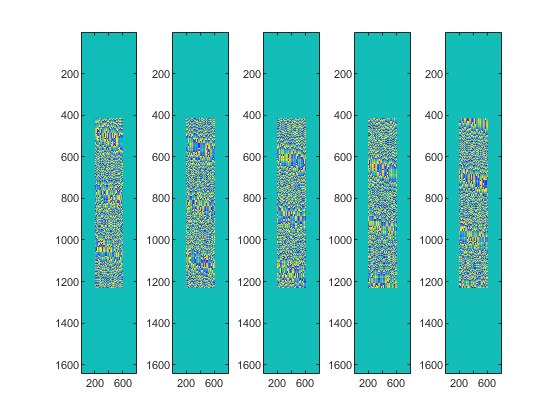
target_upsample(i, :, :) = ifft(s_f_upsample, Nr_up, 2);
subplot(1,sub_N,i);
imagesc(abs(sub_S_ftau_eta));
我这里是选择在频域补零完成升采样,需要关注的是频域补零的时候不要补到信号频率分量的中间。
合成
S_ftau_eta = zeros(Na, Nr_up);
echo_ref = squeeze(target_upsample((sub_N+1)/2, :, :));
for i = 1:sub_N
    target = squeeze(target_upsample(i, :, :));

    target = target.*(abs(echo_ref)./abs(target));
    perror = angle(echo_ref)-angle(target);
    target = target.*exp(1j*perror);

    tar_ftau_eta = fft(target, Nr_up, 2);
    tar_ftau_eta = tar_ftau_eta.*exp(2j*pi*(i-(sub_N+1)/2)*5.095*(1/(Fr*uprate)).*mat_f_tau_upsample);
    target = ifft(tar_ftau_eta, Nr_up, 2);

    target_shift = target.*exp(2j*pi*(i-(sub_N+1)/2)*step_f.*mat_t_tau_upsample);

    tar_ftau_eta = fft(target_shift, Nr_up, 2);

    S_ftau_eta = tar_ftau_eta+S_ftau_eta;
end
合成前需要补偿仍然存在相位误差,幅度误差与时延误差,同时保证相位的连续性,降低栅瓣。这里我先将所有子带的相位,幅度保持一致,然后对每个子带相位进行微调,完成补偿。我现在的微调操作是手动微调,其实可以加入优化算法,以图像对比度为目标,微调子带相位。
最后是显示
[~, a_f_pos] = max(max(abs(S_ftau_eta), [], 2));
figure("name", "频域");
plot(1:Nr_up, abs(S_ftau_eta(a_f_pos, :)));
S_tau_eta = ifft(S_ftau_eta, Nr_up, 2);
figure('name', "脉冲对比");
target_one = echo_ref;
% target_one = imrotate(target_one, rad2deg(theta_rc), 'bilinear', 'crop');
[~, a_pos] = max(max(abs(target_one), [], 2));
[~, r_pos] = max(max(abs(target_one), [], 1));
plot_range = r_pos-Nr/2:r_pos+Nr/2;
plot_range = plot_range+(max(1-plot_range(1),1));
target_plot = abs(target_one(a_pos, plot_range));
target_plot = (target_plot-min(target_plot))/(max(target_plot)-min(target_plot));
% S_tau_eta = imrotate(S_tau_eta, rad2deg(theta_rc), 'bilinear', 'crop');
S_tau_eta_plot = abs(S_tau_eta(a_pos, plot_range));
S_tau_eta_plot = (S_tau_eta_plot-min(S_tau_eta_plot))/(max(S_tau_eta_plot)-min(S_tau_eta_plot));
S_tau_eta_db = 20*log10(S_tau_eta_plot);
target_db = 20*log10(target_plot);
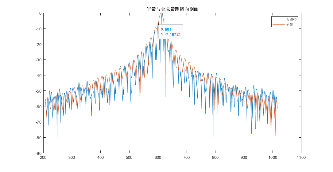
plot(plot_range, S_tau_eta_db);
hold on;
plot(plot_range, target_db);
legend("合成带","子带");
figure("name","最终效果");
imagesc(abs(S_tau_eta));
最终结果
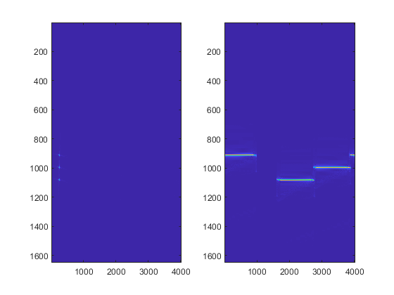
无附加的干扰噪声。
子带回波
合成频带
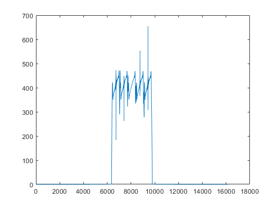
这里可以看出子带合成的效果不是很好,还可以继续加入算法来实现更好的子带合成效果。
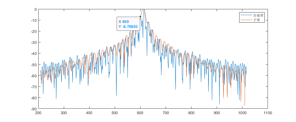
子带与合成带脉冲对比
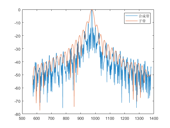
这里有比较明显的栅瓣。
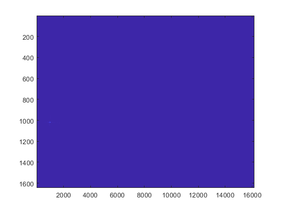
点目标成像
优化
根据论文,我在子带相位微调那,使用模拟退火进行优化。目标函数为
    function y = syn_and_image(coef, subband, sub_N, Na, Nr_up, mat_f_tau_upsample, mat_t_tau_upsample, step_f, Fr, uprate)
    S_ftau_eta = zeros(Na, Nr_up);

    for i = 1:sub_N
        target = squeeze(subband(i, :, :));

        tar_ftau_eta = fft(target, Nr_up, 2);
        tar_ftau_eta = tar_ftau_eta.*exp(2j*pi*coef(i)*(1/(Fr*uprate)).*mat_f_tau_upsample);
        target = ifft(tar_ftau_eta, Nr_up, 2);

        target_shift = target.*exp(2j*pi*(i-(sub_N+1)/2)*step_f.*mat_t_tau_upsample);

        tar_ftau_eta = fft(target_shift, Nr_up, 2);

        S_ftau_eta = tar_ftau_eta+S_ftau_eta;
    end
    target = ifft(S_ftau_eta, Nr_up, 2);
    y = max(var(20*log10(abs(target))));
    y = -y;
end
将子带数调为3,优化代码为
options = optimoptions('simulannealbnd','PlotFcns',...
          {@saplotbestx,@saplotbestf,@saplotx,@saplotf});
obj_f = @(coef)syn_and_image(coef, target_upsample, sub_N, Na, Nr_up, mat_f_tau_upsample, mat_t_tau_upsample, step_f, Fr, uprate);

[x,fval,exitFlag,output] = simulannealbnd(obj_f,[-10,0,5],[-10,0,0],[0,0,10],options);

coef = x;
在3个子带时,求解速度缓慢(可能和我的电脑有问题),求解结果为
coef=[-3.0740,0,3.0820];
求解过程
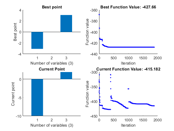
可以看出,局部最优解比较多。
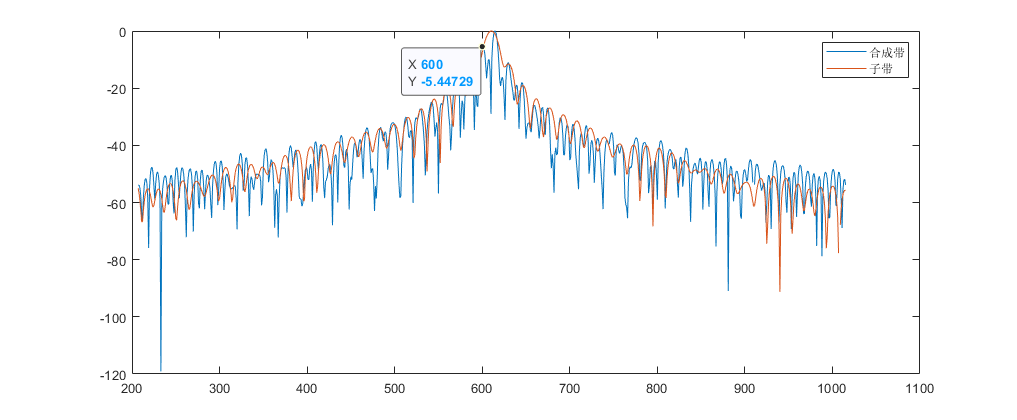
求解效果
优化空间依旧比较多。
距离压缩->子带合成->RCMC->方位压缩
这种我没有成像成功。频移子带时,好像改变的方位向的相位,导致其方位向压缩时处于不同的位置。